What Is a Cubic Equation? The Complete Beginner's Guide

Introduction

If you have studied algebra, you are likely familiar with linear equations (which form straight lines) and quadratic equations (which form U-shaped parabolas). But what happens when you take algebra one step further? You enter the fascinating world of the cubic equation.

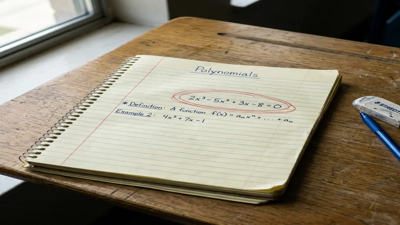
So, what is a cubic equation? In simple terms, a cubic equation is a mathematical expression where the highest power of the unknown variable is 3. These equations generate distinctive S-shaped curves on a graph and possess unique mathematical properties that set them apart from lower-degree polynomials.

Cubic equations are immensely important in both pure mathematics and practical fields. They are the mathematical engines behind many phenomena in physics, engineering, economics, and computer graphics. Any time volume is calculated, or when an object moves through three-dimensional space, cubic relationships are often at play.

Who should read this guide? This comprehensive guide is designed for everyone. Whether you are a high school student learning algebra for the first time, a college student reviewing calculus concepts, a teacher looking for resources, or simply a math enthusiast, this article is for you.

What readers will learn: By the end of this guide, you will fully understand how to define a cubic equation, recognize its standard form, identify its core characteristics, and interpret its graph. You will also learn how to differentiate it from other polynomials, discover its fascinating history, explore real-world applications, and work through numerous step-by-step examples and practice problems.

---

What Is a Cubic Equation?

Let us establish a solid foundation. A cubic equation is a polynomial equation of degree 3.

But what does that mean? In algebra, a polynomial is an expression consisting of variables and coefficients, involving operations of addition, subtraction, multiplication, and non-negative integer exponents. The “degree” of a polynomial refers to the highest exponent attached to any variable in the equation.

Therefore, it is called a third-degree equation because the highest power (or exponent) of the variable $x$ is exactly 3. You will always see an $x^3$ term in a cubic equation.

The Standard Form of a Cubic Equation

To study cubic equations systematically, mathematicians use a general template known as the standard form of a cubic equation:

$ax^3 + bx^2 + cx + d = 0$

Let us break down every variable and component in this standard form:

1. $a$: This is the leading coefficient. It is the number multiplying the $x^3$ term. It determines the overall width and directional flow (end behavior) of the graph.
2. $b$: This is the coefficient of the quadratic term ($x^2$). It influences the position of the curve’s peaks and valleys.
3. $c$: This is the coefficient of the linear term ($x$). It affects the slope of the curve as it passes through the y-intercept.
4. $d$: This is the constant term. It is a number without any variable attached. It determines exactly where the graph intersects the y-axis (the y-intercept).
5. $x$: This is the variable, or the unknown value we typically want to solve for.

Why ‘a’ Cannot Equal Zero

There is one absolutely critical rule for a cubic equation: $a \neq 0$. If $a$ were equal to zero, the $x^3$ term would vanish ($0 \cdot x^3 = 0$). The equation would then become $bx^2 + cx + d = 0$, which is a quadratic equation, not a cubic one. The presence of $x^3$ is what makes the equation cubic, so the leading coefficient $a$ must always be a non-zero number. The other coefficients ($b$, $c$, and $d$) are perfectly allowed to be zero.

Simple Examples of Cubic Equations

Here are a few quick examples to help you identify a cubic equation:

• $2x^3 - 4x^2 + 5x - 1 = 0$ (Standard form, all terms present)
• $x^3 - 8 = 0$ (Here, $a=1, b=0, c=0, d=-8$)
• $-5x^3 + x = 0$ (Here, $a=-5, b=0, c=1, d=0$)

---

History of Cubic Equations

The story of the cubic equation is one of the most dramatic and competitive chapters in the history of mathematics.

Ancient Mathematics

The quest to solve cubic equations spans thousands of years. The ancient Babylonians (around 2000 BC) created clay tablets with tables of cubes and cube roots to help them approximate solutions to basic cubic problems. The ancient Greeks, notably Archimedes, solved specific geometric problems that we now recognize as cubic equations, usually by finding the intersection of conic sections like parabolas and hyperbolas. However, they lacked the algebraic notation we use today.

Islamic Mathematics

During the Islamic Golden Age in the 11th century, the brilliant Persian mathematician and poet Omar Khayyam made massive leaps forward. He systematically classified different types of cubic equations and found geometric solutions for them by intersecting parabolas with circles. While he could not find a purely algebraic formula, his geometric methods were revolutionary.

The Renaissance and the Italian Mathematicians

The true breakthrough occurred during the Italian Renaissance in the 16th century. In 1515, Scipione del Ferro found a method to algebraically solve a specific type of cubic equation (a depressed cubic, which lacks the $x^2$ term). He kept his method a secret to win mathematical duels, a common practice at the time.

After del Ferro’s death, his student Antonio Fior challenged another mathematician, Niccolò Tartaglia, to a mathematical duel. Tartaglia managed to independently discover the solution to the cubic equation and easily defeated Fior.

The drama escalated when Gerolamo Cardano, a prominent polymath, convinced Tartaglia to share his secret method under an oath of secrecy. Cardano later learned of del Ferro’s earlier discovery and felt this released him from his oath. In 1545, Cardano published the method in his landmark book, Ars Magna.

Cardano’s student, Lodovico Ferrari, used these findings to solve the quartic (fourth-degree) equation. Ultimately, solving cubic equations forced mathematicians to confront the concept of the square root of negative numbers, giving birth to the entirely new field of complex numbers. Solving the cubic equation wasn’t just a mathematical trick; it forever expanded the boundaries of human knowledge.

---

Characteristics of Cubic Equations

Understanding the properties of cubic equations allows you to predict how they behave mathematically and visually. Here are the defining characteristics:

1. Degree: The highest exponent is always 3.
2. Maximum Number of Roots: The Fundamental Theorem of Algebra states that a polynomial of degree $n$ has exactly $n$ roots. Therefore, every cubic equation has exactly 3 roots (also called zeros or solutions).
3. Possible Real and Complex Roots: Because the coefficients in standard real-world cubic equations are real numbers, complex roots must occur in conjugate pairs. This means a cubic equation can have:
   • 3 real roots (distinct or repeating)
   • 1 real root and 2 complex roots Crucially, a cubic equation will ALWAYS have at least one real root. This is because the graph must cross the x-axis at least once.
4. Odd-Degree Polynomial Behavior: Because 3 is an odd number, cubic equations exhibit odd-degree polynomial behavior. The opposite ends of the graph will always head in opposite vertical directions.
5. End Behavior:
   • If the leading coefficient ($a$) is positive, the graph goes down to the left (towards negative infinity) and up to the right (towards positive infinity).
   • If the leading coefficient ($a$) is negative, the graph goes up to the left (towards positive infinity) and down to the right (towards negative infinity).
6. Turning Points: A turning point is where the graph changes direction (from going up to going down, or vice versa), creating a local peak (maximum) or valley (minimum). A polynomial of degree $n$ can have at most $n - 1$ turning points. Thus, a cubic equation can have at most 2 turning points. Sometimes, it has 0 turning points, just flattening out momentarily before continuing its path.
7. Inflection Point: Every cubic equation has exactly one inflection point. This is the exact point on the curve where the concavity changes (shifting from curving downward like a frown to curving upward like a smile, or vice versa). It represents the point of maximum or minimum slope.
8. Continuity: Like all polynomial functions, a cubic function is continuous. There are no breaks, holes, or vertical asymptotes anywhere on the graph.
9. Graph Shape: The graph is generally S-shaped or a continuous curve that spans from negative infinity to positive infinity along the y-axis.

Comparison Table of Cubic Characteristics

Characteristic	Property / Rule for Cubic Equations
Degree	Always 3
Total Roots	Exactly 3 (Real + Complex combined)
Real Roots	At least 1, up to 3
Complex Roots	0 or 2 (Must appear in conjugate pairs)
Turning Points	Maximum of 2 (can be 0)
Inflection Points	Exactly 1
End Behavior ($a > 0$)	Down on left, Up on right
End Behavior ($a < 0$)	Up on left, Down on right

---

Standard Form of a Cubic Equation

To work mathematically with cubics, we must structure them properly. We use different terminologies to describe these structures.

1. General Form

The general form is the standard way to write the equation, arranged in descending order of the exponents (from largest to smallest).
Formula: $ax^3 + bx^2 + cx + d = 0$
Example: $4x^3 - 7x^2 + 2x - 9 = 0$

2. Standard Form

“General form” and “standard form” are often used interchangeably in algebra. Both refer to $ax^3 + bx^2 + cx + d = 0$. Writing an equation in standard form makes it easy to identify the coefficients $a, b, c$, and $d$.

3. Monic Cubic Equation

A monic cubic equation is a specific type of standard form where the leading coefficient ($a$) is equal to 1. Monic polynomials are generally easier to factor and work with.
Formula: $x^3 + bx^2 + cx + d = 0$
Example: $x^3 - 5x^2 + 8x - 4 = 0$

4. Depressed Cubic Equation

A depressed cubic equation is a cubic equation that is missing its squared term. In other words, the coefficient $b$ is exactly zero. This form is historically incredibly important, as Cardano’s method relies on converting any standard cubic into a depressed cubic to solve it.
Formula: $ax^3 + cx + d = 0$
Example: $2x^3 - 15x + 7 = 0$

---

Types of Cubic Equations

Based on their structure and their roots, cubic equations can be categorized into several distinct types.

1. General Cubic

This is the full equation containing all terms: $ax^3 + bx^2 + cx + d = 0$.
Example: $3x^3 + 2x^2 - x + 5 = 0$

2. Monic Cubic

The leading coefficient $a$ is 1.
Example: $x^3 + 6x^2 + 11x + 6 = 0$

3. Depressed Cubic

The $x^2$ term is missing ($b = 0$).
Example: $x^3 - 7x + 6 = 0$

4. Factored Cubic

The cubic expression is broken down into a product of linear binomials. This is incredibly useful for instantly identifying the roots of the equation.
Formula: $a(x - r_1)(x - r_2)(x - r_3) = 0$
Example: $2(x - 1)(x + 3)(x - 4) = 0$ (Here, the roots are $x=1, x=-3,$ and $x=4$)

5. Perfect Cube Equations

This occurs when a binomial is cubed. It means all three roots are exactly the same number.
Formula: $(x - r)^3 = 0$
Example: $(x - 2)^3 = 0$ (This expands to $x^3 - 6x^2 + 12x - 8 = 0$. The only root is $x=2$ with a multiplicity of 3).

6. Repeated Root Cubic Equations

These are equations where two of the three roots are identical. On a graph, this causes the curve to “touch” the x-axis and bounce off, rather than crossing straight through it.
Formula: $a(x - r_1)^2(x - r_2) = 0$
Example: $(x - 3)^2(x + 1) = 0$ (Roots are $x=3, x=3$, and $x=-1$)

---

Components of a Cubic Equation

To master the third-degree equation, you must be able to instantly identify its anatomical components. Let’s look at the equation $f(x) = -4x^3 + 7x^2 - x + 12$.

1. Leading Coefficient: The number attached to the $x^3$ term.
   • In our example: -4
2. Constant Term: The number with no variable. This is always the y-intercept.
   • In our example: 12
3. Variable: The unknown letter we are evaluating or solving for.
   • In our example: $x$
4. Coefficients: The numerical multipliers for every variable term.
   • In our example: -4, 7, and -1 (Note that $-x$ implies a coefficient of -1).
5. Exponents: The powers to which the variables are raised.
   • In our example: 3, 2, and an implied 1 on the linear term.
6. Polynomial Degree: The highest exponent in the whole expression.
   • In our example: 3

Worked Example: Identifying Components

Problem: Identify all components of $5x^3 - 9 = 0$.
Solution:

• Rewrite in standard form: $5x^3 + 0x^2 + 0x - 9 = 0$
• Leading coefficient ($a$): $5$
• Quadratic coefficient ($b$): $0$
• Linear coefficient ($c$): $0$
• Constant term ($d$): $-9$
• Degree: $3$

---

Graph of a Cubic Equation

The graph of a cubic equation, $y = ax^3 + bx^2 + cx + d$, is a curved line called a cubic parabola or an S-curve. Learning to read this graph is essential for calculus and advanced algebra.

Shape

The defining feature of a cubic graph is its “S” shape. Because $x^3$ can produce very large negative numbers (when $x$ is negative) and very large positive numbers (when $x$ is positive), the graph extends to infinity in both vertical directions.

End Behavior

The leading coefficient $a$ acts as the steering wheel for the graph’s ends.

• Positive Leading Coefficient ($a > 0$): As you read the graph from left to right, it starts from the bottom left quadrant, snakes its way through the middle, and exits toward the top right quadrant.
• Negative Leading Coefficient ($a < 0$): As you read from left to right, it starts from the top left quadrant, snakes through the middle, and exits toward the bottom right quadrant.

X-Intercepts

The x-intercepts are where the graph crosses the horizontal x-axis. These exact points are the roots (or solutions) of the cubic equation.

• A cubic graph must cross the x-axis at least once.
• It can cross it a maximum of three times.

Y-Intercept

The graph will cross the vertical y-axis exactly once. This point is entirely dictated by the constant term $d$. If the equation is $y = 2x^3 + x^2 - 4x + 7$, the graph will intersect the y-axis exactly at $(0, 7)$.

Turning Points

These are local maximums (peaks) or local minimums (valleys).

• A cubic graph can have two turning points (a distinct peak and a valley).
• Or, it can have zero turning points (it flattens briefly but keeps heading in the same general vertical direction). It is impossible for a cubic to have exactly one turning point; it must have two or zero.

Inflection Point

Smack in the middle of the graph, between the two turning points, is the inflection point. This is the exact center of the “S” curve where the concavity flips. Every cubic graph possesses exactly one point of inflection, and interestingly, every cubic graph has perfect point-symmetry centered exactly on this inflection point.

---

Roots of a Cubic Equation

The “roots” of a cubic equation $ax^3 + bx^2 + cx + d = 0$ are the values of $x$ that make the equation true. They are the locations where the graph intersects the x-axis. As established, there are always 3 roots, but their nature can vary.

Real Roots

A real root is a standard number (whole, fraction, decimal, rational, or irrational) where the graph visibly crosses the x-axis. Every cubic equation has at least one real root because the line must get from negative infinity to positive infinity, forcing it to cross the horizontal axis.

Complex Roots

Complex roots involve the imaginary unit $i$ (where $i = \sqrt{-1}$). If a graph crosses the x-axis only once, the remaining two roots are complex numbers. Complex roots do not show up as x-intercepts on a standard Cartesian plane. Because the coefficients of our polynomial are real numbers, complex roots must occur in conjugate pairs (e.g., $2 + 3i$ and $2 - 3i$). You can never have exactly one or exactly three complex roots in an equation with real coefficients.

Repeated Roots

Sometimes, the math yields the same number twice.

• Double Root: The graph touches the x-axis at the root and “bounces” back in the direction it came from, creating a turning point exactly on the axis. This accounts for two of the three roots. The curve will then cross the axis somewhere else for the third root.
• Triple Root: Also known as a multiplicity of 3. The graph passes through the x-axis, but it “flattens out” right as it crosses. It serves as the root, the inflection point, and a saddle point all at once. Example: $x^3 = 0$ has a triple root at $x = 0$.

The Discriminant

Just like quadratic equations have a discriminant ($b^2 - 4ac$) that tells you the nature of the roots, cubic equations have a discriminant ($\Delta$) too. While the formula is complex ($\Delta = 18abcd - 4b^3d + b^2c^2 - 4ac^3 - 27a^2d^2$), it follows simple rules:

• If $\Delta > 0$, the equation has 3 distinct real roots.
• If $\Delta = 0$, the equation has multiple roots (all roots are real, but at least two are the same).
• If $\Delta < 0$, the equation has 1 real root and 2 complex conjugate roots.

---

How to Recognize a Cubic Equation

Identifying a cubic equation is a matter of looking for the highest exponent.

The Golden Rule

The highest exponent attached to any variable must be exactly 3. If there is an $x^4$, it is not a cubic. If the highest is $x^2$, it is not a cubic. The leading coefficient for the $x^3$ term cannot be zero.

Identification Practice Table

Equation	Is it Cubic?	Reason
$4x^3 - 2x^2 + x - 1 = 0$	Yes	Highest power is 3.
$x^3 = 125$	Yes	Highest power is 3 (this is $x^3 - 125 = 0$).
$7x^2 - 5x + 2 = 0$	No	Highest power is 2. This is a quadratic equation.
$0x^3 + 5x^2 - 1 = 0$	No	The $x^3$ term is multiplied by 0, leaving only a quadratic.
$x(x^2 + 4) = 0$	Yes	When expanded, it becomes $x^3 + 4x = 0$. Highest power is 3.
$3x^4 - x^3 = 0$	No	Highest power is 4. This is a quartic equation.
$y = x^3 + \frac{1}{x}$	No	$\frac{1}{x}$ is $x^{-1}$. Polynomials cannot have negative exponents.

---

How Cubic Equations Differ from Other Polynomial Equations

To truly grasp the cubic polynomial, you must see how it sits in the hierarchy of mathematical functions.

Polynomial Comparison Table

Feature	Linear	Quadratic	Cubic	Quartic
Highest Degree	1 ($ax + b$)	2 ($ax^2 + \dots$)	3 ($ax^3 + \dots$)	4 ($ax^4 + \dots$)
Max Number of Roots	1	2	3	4
Max Turning Points	0	1	2	3
Graph Shape	Straight Line	Parabola (U-shape)	S-Curve	W-shape or U-shape
Guaranteed Real Root?	Yes (1)	No (Could be 0)	Yes (At least 1)	No (Could be 0)
Inflection Points	0	0	Exactly 1	0 or 2
Common Solving Method	Basic Algebra	Quadratic Formula	Factoring, Synthetic Div.	Factoring, Ferrari’s Method

Key Takeaways:

1. Odd vs. Even Degrees: Linear (degree 1) and Cubic (degree 3) graphs have opposite end behaviors, meaning they start low and end high (or vice versa), guaranteeing they cross the x-axis. Quadratic (degree 2) and Quartic (degree 4) graphs start and end in the same vertical direction (both pointing up or both pointing down), meaning they might float entirely above or below the x-axis and have zero real roots.
2. Complexity: While linear and quadratic equations have simple, universally taught formulas, solving the general cubic equation requires much more advanced techniques (like Cardano’s formula), representing a massive jump in mathematical complexity.

---

Common Methods Used to Solve Cubic Equations

Solving a cubic equation means finding the values of $x$ that make the equation equal to zero. Unlike the quadratic formula, which is a single plug-and-play equation, solving a cubic often requires a toolkit of different strategies depending on the equation’s structure.

1. Factoring by Grouping

If the cubic equation has four terms, you can sometimes split it down the middle, factor out the greatest common factor from the first two terms, do the same for the last two terms, and find a common binomial.
Use when: The ratio of the first two coefficients matches the ratio of the last two.

2. Factoring the Sum or Difference of Cubes

If the equation consists of only two terms, and both are perfect cubes (e.g., $x^3 - 8 = 0$ or $x^3 + 27 = 0$), there are specific formulas to factor them immediately:

• Difference: $a^3 - b^3 = (a - b)(a^2 + ab + b^2)$
• Sum: $a^3 + b^3 = (a + b)(a^2 - ab + b^2)$

3. The Rational Root Theorem

This theorem helps you list all possible rational roots (fractions and integers) of a polynomial. You take the factors of the constant term ($d$) and divide them by the factors of the leading coefficient ($a$). You then test these possibilities (using synthetic division) to find a real root.

4. Synthetic Division and Polynomial Long Division

Once you find one root (let’s say $x = r$) using the Rational Root Theorem or by guessing, you divide the cubic polynomial by $(x - r)$. This division yields a quadratic equation. You can then easily solve the remaining quadratic equation using the quadratic formula or standard factoring to find the final two roots.

5. Cardano’s Method

If an equation cannot be easily factored and has no rational roots, you must use Cardano’s algebraic method. This is a highly advanced technique that involves substituting variables to remove the $x^2$ term (creating a depressed cubic) and then applying a complex geometric-algebraic formula to extract the roots.

6. Graphing and Calculator Methods

In the modern world, the most common way to solve complex, messy real-world cubic equations is via graphing calculators or computational software (like Desmos, WolframAlpha, or Python). By graphing the function, the roots are visually identifiable as the precise x-intercepts.

---

Real World Applications

Why do we force students to learn about cubic equations? Because the real world operates in three dimensions, and mathematical models of reality frequently require third-degree powers.

1. Engineering and Fluid Mechanics

When designing ships or submarines, engineers use cubic equations to model the relationship between a vessel’s hull shape, its buoyancy, and fluid resistance. The drag force exerted on moving objects in a fluid often scales non-linearly, requiring polynomials of degree 3 to approximate flow dynamics accurately.

2. Architecture and Construction

Architects use cubic functions to design smooth curves. When laying out modern curving structures, bridges, or aesthetic arches, structural engineers use cubic splines (piecing together multiple cubic equations) to ensure the curves are perfectly smooth and continuous without abrupt changes in slope.

3. Computer Graphics and Animation

If you play 3D video games or watch animated movies, you are looking at cubic equations. To make a character move smoothly from point A to point B, software uses “Bézier curves” and “Cubic Splines”. These equations calculate the precise curved path an object or camera should take, ensuring the motion looks organic rather than robotic.

4. Physics and Electrical Engineering

In thermodynamics, the “equations of state” (like the Van der Waals equation) which predict how real gases behave under changing pressure, volume, and temperature, are cubic equations in terms of volume. In electricity, the voltage-current characteristics of certain non-linear components (like tunnel diodes) are modeled using cubic functions.

5. Economics and Business

Economists use cubic equations to model cost functions. A typical manufacturing cost curve might start steep, flatten out as the factory reaches maximum efficiency (economies of scale), and then steepen again as the factory becomes overcrowded and overworked. This S-curve behavior is perfectly modeled by a cubic function.

6. Robotics and Machine Learning

Roboticists use cubic polynomials to program the trajectories of robotic arms. If an arm needs to pick up an object and place it elsewhere, a cubic equation ensures that the arm accelerates smoothly, reaches peak velocity, and decelerates smoothly to a stop, preventing jerky movements that could damage the robot.

---

Common Mistakes When Working with Cubic Equations

When students begin working with cubic equations, several common pitfalls occur.

1. Confusing Cubic with Quadratic

The most common mistake is trying to apply quadratic rules to a cubic problem. Students often instinctively try to use the quadratic formula ($x = \frac{-b \pm \sqrt{b^2 - 4ac}}{2a}$) on a cubic equation. The quadratic formula only works for $ax^2 + bx + c = 0$. It will not solve an $x^3$ equation.

2. Forgetting the Highest Exponent

When equations are not written in standard descending order (e.g., $4x^2 + 5x^3 - 2 = 0$), students sometimes mistakenly look at the first term ($4x^2$) and assume the equation is quadratic. Always scan the entire equation to locate the highest exponent before identifying it.

3. Misidentifying Coefficients

If an equation is missing a term, students often assign the wrong value to $a, b, c,$ or $d$. For example, in $x^3 - 5x + 2 = 0$, the $x^2$ term is missing.
Incorrect: $a=1, b=-5, c=2$.
Correct: $a=1, b=0, c=-5, d=2$. Failing to place a zero for missing terms ruins synthetic division and formulas.

4. Forgetting the Rule of Three Roots

Students often factor a cubic, find one real root, and stop, thinking they have finished the problem. A cubic equation always has three roots. If you find one real root, you must divide the polynomial to find the remaining quadratic, and solve that quadratic to find the final two roots (even if they are complex numbers).

5. Sign Errors During Grouping

When factoring by grouping, distributing negative signs incorrectly is a frequent source of calculation mistakes. Always double-check your algebraic expansions.

---

Worked Examples

Let us cement your understanding by solving several types of cubic equations, step-by-step.

Beginner Examples

Example 1: Solving a Simple Factored Cubic Solve: $(x - 2)(x + 5)(x - 1) = 0$
Step 1: Use the Zero Product Property. If things multiply to equal zero, at least one of them must be zero.
Step 2: Set each factor to zero. $x - 2 = 0 \rightarrow x = 2$ $x + 5 = 0 \rightarrow x = -5$ $x - 1 = 0 \rightarrow x = 1$
Solution: $x = 2, x = -5, x = 1$

Example 2: Solving by Factoring out the Greatest Common Factor (GCF) Solve: $x^3 - 4x = 0$
Step 1: Notice both terms share an $x$. Factor it out. $x(x^2 - 4) = 0$
Step 2: Notice that $(x^2 - 4)$ is a difference of squares. Factor it. $x(x - 2)(x + 2) = 0$
Step 3: Set each factor to zero.
Solution: $x = 0, x = 2, x = -2$

Example 3: Difference of Cubes Solve: $x^3 - 64 = 0$
Step 1: Recognize this fits the pattern $a^3 - b^3$. Here, $a=x$ and $b=4$ (since $4^3 = 64$).
Step 2: Use the formula $(a - b)(a^2 + ab + b^2) = 0$. $(x - 4)(x^2 + 4x + 16) = 0$
Step 3: First root is $x = 4$.
Step 4: Solve the quadratic part using the quadratic formula: $x = \frac{-4 \pm \sqrt{16 - 4(1)(16)}}{2} = \frac{-4 \pm \sqrt{-48}}{2} = \frac{-4 \pm 4i\sqrt{3}}{2} = -2 \pm 2i\sqrt{3}$
Solution: $x = 4$, and $x = -2 + 2i\sqrt{3}$, and $x = -2 - 2i\sqrt{3}$

Example 4: Solving a Perfect Cube Solve: $x^3 - 9x^2 + 27x - 27 = 0$
Step 1: Recognize this is the expansion of $(x - 3)^3$.
Step 2: $(x - 3)^3 = 0$
Step 3: Take the cube root of both sides. $x - 3 = 0$
Solution: $x = 3$ (This is a root with a multiplicity of 3).

Intermediate Examples

Example 5: Factoring by Grouping Solve: $x^3 + 2x^2 - 9x - 18 = 0$
Step 1: Group the first two terms and the last two terms. $(x^3 + 2x^2) - (9x + 18) = 0$
Step 2: Factor out the GCF from each group. $x^2(x + 2) - 9(x + 2) = 0$
Step 3: Factor out the common binomial $(x + 2)$. $(x + 2)(x^2 - 9) = 0$
Step 4: Factor the difference of squares. $(x + 2)(x - 3)(x + 3) = 0$
Solution: $x = -2, x = 3, x = -3$

Example 6: Grouping with a Leading Coefficient Solve: $2x^3 - 3x^2 - 8x + 12 = 0$
Step 1: Group. $(2x^3 - 3x^2) - (8x - 12) = 0$
Step 2: Factor GCF. $x^2(2x - 3) - 4(2x - 3) = 0$
Step 3: Factor out binomial. $(2x - 3)(x^2 - 4) = 0$
Step 4: Expand difference of squares. $(2x - 3)(x - 2)(x + 2) = 0$
Solution: $x = 1.5, x = 2, x = -2$

Example 7: Using the Rational Root Theorem (Part 1) Solve: $x^3 - 4x^2 + x + 6 = 0$
Step 1: Identify possible roots. Factors of constant (6) / Factors of leading coefficient (1). Possible roots: $\pm 1, \pm 2, \pm 3, \pm 6$.
Step 2: Test $x = -1$ using substitution. $(-1)^3 - 4(-1)^2 + (-1) + 6 = -1 - 4 - 1 + 6 = 0$. Yes, $x = -1$ is a root.
Step 3: Use synthetic division. Divide the polynomial by $(x + 1)$. Coefficients: 1, -4, 1, 6. Root: -1. The result is $x^2 - 5x + 6 = 0$.
Step 4: Factor the remaining quadratic. $(x - 2)(x - 3) = 0$.
Solution: $x = -1, x = 2, x = 3$

Example 8: Using the Rational Root Theorem (Part 2) Solve: $x^3 - 7x - 6 = 0$
Step 1: Possible roots: $\pm 1, \pm 2, \pm 3, \pm 6$.
Step 2: Test $x = -1$. $(-1)^3 - 7(-1) - 6 = -1 + 7 - 6 = 0$. Root found: $x = -1$.
Step 3: Synthetic division by $(x + 1)$. Important: the $x^2$ coefficient is 0. Coefficients: 1, 0, -7, -6. Root: -1. Result: $x^2 - x - 6 = 0$.
Step 4: Factor quadratic. $(x - 3)(x + 2) = 0$.
Solution: $x = -1, x = 3, x = -2$

Advanced Examples

Example 9: Rational Root Theorem with Complex Roots Solve: $x^3 - 2x^2 + x - 2 = 0$
Step 1: Grouping works here! $(x^3 - 2x^2) + (x - 2) = 0$
Step 2: $x^2(x - 2) + 1(x - 2) = 0$
Step 3: $(x - 2)(x^2 + 1) = 0$
Step 4: First root is $x = 2$.
Step 5: Solve $x^2 + 1 = 0 \rightarrow x^2 = -1 \rightarrow x = \pm i$
Solution: $x = 2, x = i, x = -i$ (One real root, two complex conjugate roots).

Example 10: Using Quadratic Formula after Division Solve: $x^3 - 5x^2 + 8x - 6 = 0$
Step 1: Test roots from factors of 6. Test $x = 3$. $3^3 - 5(3^2) + 8(3) - 6 = 27 - 45 + 24 - 6 = 0$. Yes, $x=3$ is a root.
Step 2: Synthetic division of $x^3 - 5x^2 + 8x - 6$ by 3. Result: $x^2 - 2x + 2 = 0$.
Step 3: This quadratic does not factor. Use quadratic formula. $x = \frac{2 \pm \sqrt{4 - 4(1)(2)}}{2} = \frac{2 \pm \sqrt{-4}}{2} = \frac{2 \pm 2i}{2} = 1 \pm i$
Solution: $x = 3, x = 1 + i, x = 1 - i$

Example 11: A messy leading coefficient Solve: $2x^3 - 5x^2 - 14x + 8 = 0$
Step 1: Rational Root Theorem. Factors of 8 over factors of 2. Possible roots include $\pm 1, \pm 2, \pm 4, \pm 8, \pm 1/2$.
Step 2: Test $x = 4$. $2(64) - 5(16) - 14(4) + 8 = 128 - 80 - 56 + 8 = 0$. Root is $x=4$.
Step 3: Synthetic Division by 4. Coefficients: 2, -5, -14, 8. Root: 4. Result: $2x^2 + 3x - 2 = 0$.
Step 4: Factor the quadratic: $(2x - 1)(x + 2) = 0$. Roots are $x = 1/2, x = -2$.
Solution: $x = 4, x = 1/2, x = -2$

Example 12: Graph Interpretation Question: You are looking at a graph of a cubic polynomial $y = ax^3 + bx^2 + cx + d$. The graph starts at the top left, crosses the x-axis at -3, touches the x-axis at 2 and bounces down, and crosses the y-axis at -12. Write the factored equation.
Step 1: Start high left, end low right means leading coefficient $a$ is negative.
Step 2: Root at -3 means a factor of $(x + 3)$.
Step 3: Bouncing at 2 means a repeated root, so a factor of $(x - 2)^2$.
Step 4: Base equation is $y = a(x + 3)(x - 2)^2$.
Step 5: Use the y-intercept $(0, -12)$ to find $a$. Plug in $x=0, y=-12$. $-12 = a(0 + 3)(0 - 2)^2$ $-12 = a(3)(4)$ $-12 = 12a \rightarrow a = -1$
Solution: The equation is $y = -(x + 3)(x - 2)^2$

---

Practice Problems

Test your knowledge with these 30 practice problems! (Solutions are provided immediately after this section).

Beginner Level

1. Identify the degree of $4x^2 - x^3 + 7$.
2. Is $2x^3 - 8x + 1 = 0$ a depressed cubic?
3. What is the maximum number of turning points on a cubic graph?
4. True or False: A cubic equation can have exactly two real roots and zero complex roots.
5. Identify the constant term in $5x^3 - 3x^2 + x - 10 = 0$.
6. Solve: $(x - 7)(x + 1)(x - 4) = 0$.
7. Solve: $x^3 - x = 0$.
8. Factor: $x^3 + 8 = 0$.
9. What is the end behavior of $y = 3x^3 - 2x^2 + x$?
10. If a cubic equation has roots at $x = 2, 3,$ and $4$, write it in factored form (assume $a=1$).

Intermediate Level

11. Solve by grouping: $x^3 + 3x^2 - 4x - 12 = 0$.
12. Solve by grouping: $2x^3 - x^2 - 18x + 9 = 0$.
13. List all possible rational roots for $3x^3 + 2x^2 - 7x + 4 = 0$.
14. Use the Rational Root Theorem to solve: $x^3 - 6x^2 + 11x - 6 = 0$.
15. Solve: $x^3 + 2x^2 - x - 2 = 0$.
16. Find the roots of $x^3 - 27 = 0$.
17. If one root of $x^3 - x^2 + 4x - 4 = 0$ is $x = 1$, find the other two.
18. Determine the y-intercept of $y = -2(x - 1)(x + 2)(x - 3)$.
19. A cubic graph crosses the x-axis at 1, -1, and 5. The y-intercept is 10. Find the equation.
20. Solve: $x^4 - 8x^3 + 16x^2 = 0$. (Hint: factor first to reveal a cubic relationship).

Advanced Level

21. Solve: $x^3 - 3x^2 + 4x - 12 = 0$.
22. Solve: $2x^3 - 7x^2 + 7x - 2 = 0$.
23. Find all roots of $x^3 + 4x^2 + 6x + 4 = 0$ given that $x = -2$ is a root.
24. A cubic equation with real coefficients has roots $x = 3$ and $x = 1 - 2i$. What is the third root?
25. Write the standard form equation for the roots listed in problem 24 (assume $a=1$).
26. Solve: $x^3 - 5x^2 + 9x - 5 = 0$.
27. Given $x^3 + bx^2 + cx + d = 0$. If the roots are $p, q$, and $r$, what is the product of the roots in terms of $d$?
28. Find the intersection points of the cubic $y = x^3 - x$ and the line $y = 3x$.
29. Solve the depressed cubic $x^3 - 7x + 6 = 0$ using any method.
30. Prove that $x^3 - 2x^2 + x - 5 = 0$ has exactly one real root without fully solving it.

---

Solutions to Practice Problems

Beginner Solutions:

1. Degree is 3.
2. Yes. There is no $x^2$ term ($b=0$).
3. 2 turning points.
4. False. It can have two real roots if one is a repeated root (double root), but total roots must always sum to 3. The remaining “root” is just the repeated one. It cannot have zero complex and only two roots total.
5. -10
6. $x = 7, x = -1, x = 4$
7. $x(x^2 - 1) = 0 \rightarrow x(x-1)(x+1) = 0 \rightarrow x=0, x=1, x=-1$
8. $(x + 2)(x^2 - 2x + 4) = 0$
9. Down on the left, Up on the right (because $a = 3$, which is positive).
10. $y = (x - 2)(x - 3)(x - 4)$

Intermediate Solutions: 11. $x^2(x+3) - 4(x+3) = 0 \rightarrow (x+3)(x^2-4) = 0 \rightarrow x = -3, 2, -2$ 12. $x^2(2x-1) - 9(2x-1) = 0 \rightarrow (2x-1)(x^2-9) = 0 \rightarrow x = 1/2, 3, -3$ 13. Factors of 4 over factors of 3: $\pm 1, \pm 2, \pm 4, \pm 1/3, \pm 2/3, \pm 4/3$ 14. Roots are $x = 1, 2, 3$ 15. Grouping: $x^2(x+2) - 1(x+2) = 0 \rightarrow x = -2, 1, -1$ 16. $(x-3)(x^2+3x+9) = 0 \rightarrow x=3, x = \frac{-3 \pm 3i\sqrt{3}}{2}$ 17. Divide by $(x-1)$ to get $x^2 + 4 = 0$. Other roots: $x = 2i, -2i$ 18. Plug in $x=0$. $y = -2(-1)(2)(-3) = -12$. 19. $y = a(x-1)(x+1)(x-5)$. Plug in $(0, 10)$: $10 = a(-1)(1)(-5) \rightarrow 10 = 5a \rightarrow a = 2$. Equation: $y = 2(x-1)(x+1)(x-5)$. 20. Factor out $x^2$. $x^2(x^2 - 8x + 16) = 0 \rightarrow x^2(x-4)^2 = 0 \rightarrow x=0$ (double), $x=4$ (double).

Advanced Solutions: 21. Grouping: $x^2(x-3) + 4(x-3) = 0 \rightarrow (x-3)(x^2+4) = 0 \rightarrow x=3, 2i, -2i$. 22. Test roots. $x=1$ works. Divide by $(x-1)$ gives $2x^2 - 5x + 2 = 0 \rightarrow (2x-1)(x-2) = 0$. Roots: $1, 2, 1/2$. 23. Divide by $(x+2)$ to get $x^2 + 2x + 2 = 0$. Quadratic formula yields $x = -1 \pm i$. 24. Complex roots come in conjugate pairs. The third root must be $1 + 2i$. 25. $(x-3)(x - (1-2i))(x - (1+2i)) = (x-3)(x^2 - 2x + 5) = x^3 - 5x^2 + 11x - 15 = 0$. 26. Test $x=1$. Divide to get $x^2 - 4x + 5 = 0$. Roots: $1, 2 \pm i$. 27. The product of the roots is equal to $-d/a$. Since it’s monic ($a=1$), the product is $-d$. 28. Set them equal: $x^3 - x = 3x \rightarrow x^3 - 4x = 0 \rightarrow x(x-2)(x+2) = 0$. Points at $x = 0, 2, -2$. 29. Test roots. $x=1$ works. Divide by $(x-1)$ to get $x^2 + x - 6 = 0 \rightarrow (x+3)(x-2) = 0$. Roots: $1, -3, 2$. 30. To prove it has one real root, take the derivative: $3x^2 - 4x + 1$. Find critical points: $(3x-1)(x-1) = 0 \rightarrow x=1/3, x=1$. Test the y-values at these points. At $x=1, y = 1 - 2 + 1 - 5 = -5$ (Negative). At $x=1/3, y = 1/27 - 2/9 + 1/3 - 5$ (Also Negative). Since both turning points are below the x-axis, the graph only crosses the x-axis once (to the right of the turning points), meaning it has exactly one real root.

---

Frequently Asked Questions